How to Create a Drop-down Box in Excel

My husband called me into his office recently and asked me how to do a drop-down box in Excel.  When I finished showing him, he asked me how I knew how to do it.  I am not sure....I just do.  lol!  So, I thought I'd do a blog post on how to do it easily.  This way he can refer to my post if he needs to remember how to do it.  There are other ways of doing drop-downs, but I find this to be the easiest. 

Drop-down boxes are VERY convenient if you have to choose the same items over and over.  Since a great Coupon blog recently linked to my site and because I am just getting into the whole "couponing" thing.....I'm going to use a "Coupon" spreadsheet as my example.

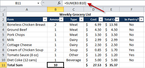
My Coupon Spreadsheet (on Sheet1):

I do not like to type things out if I don't have to.  I would rather click a drop down or just type the first letter.  With drop-downs you can do either.

I'm going to create the items for my drop-down on a different sheet than my actual coupon sheet.  If you have a blank "Sheet2" sheet at the bottom of your workbook this is where we will create the drop-down items.  If your Sheet2 is not blank just add a new sheet by right-clicking a sheet and choosing Insert...and then worksheet.  Now, I've created two columns on Sheet2.  One column with my "Store" names and one with my "Coupon Price".  These items will be what shows up in my drop-down when I click it from my main spreadsheet.

Now that I have the items in my drop-down entered into my Sheet2 I will need to tell Excel that these are the items I want to use in my first drop-down.  Highlight the store names (do not include the header) and then click on the Formulas ribbon/toolbar and choose Define Name (see below).

Now, I want to give my drop-down list a name.  I named mine "store" and then click OK.  The items in "Scope" and "Refers to" will be automatically entered for you.

Now, do the same thing for the "Coupon Price" items in column B of Sheet2.  Highlight the price items in column B (do not highlight the header), click on Define Name and then name your drop-down list.

You should now have both of your drop-down lists named.  Go to your original sheet (mine is Sheet1).  Now, highlight column C, then click on the Data ribbon/toolbar and choose Data Validation.

This is where we tell Excel what drop-down list we want it to use for column C.  Once the Data Validation window opens choose "List" in the Allow field (see orange arrow below).  Then, tell it your list source (red arrow) which we named "store" earlier.  You will need to enter an "=" before your source name.  So, it will be "=store". Click OK.

Now, when you click on a cell in column C you will have your drop-down list of stores available to you.

For column B you will do the same thing.  Highlight column B, choose Data Validation, choose List from the drop-down and then enter in "=" followed by what you named your second drop-down list earlier.  You will see below that we now have our second drop-down with our list of coupon amounts.  You can either click the button on the drop-down to add your items or just type the first few letters/amounts and it will pop-up with your item.

This was VERY easy.  Here is my spreadsheet all filled in.  I am all ready to go to the store. I am all done and it is ready for me to reuse next time!

If you need to add items to your drop-downs at a later time it is very easy.  Go to your spreadsheet where you listed out your drop-down items.  In the steps above our sheet was sheet2.  Add your items.  Then,  click on the Name Manager button on your Formulas ribbon/toolbar.

Once it pops up with your name manager, highlight which list you need to update followed by the Edit... button.

It will pop up with the Edit Name window (below).  You would just need to change your "Refers to" location to include the new rows of items.  If your data ended at A8 before and now it is A10.  Just change the $A$8 to $A$10 and you will now have the new items in your drop-down box.

Thank you for reading my Tech blog!  Good luck!

Excel (Combining or Separating Data in Columns)

Are you ever working in a spreadsheet and need to combine two columns or separate two columns? Below you will find the instructions on how to add two columns together as well as how to separate two columns to meet your needs. 

Let's pretend we have a spreadsheet that contains the information for 300 of our clients.  We would like to pull together a mailing list, but the Last Name and First Name fields are separated.  We would need to combine them.  Of course we can do this automatically in Word using a Mail Merge, but lets just say for this example that is not an option.

Below is an example of our spreadsheet.

We need to add a blank column to column C (to do this, highlight column C, right-click and choose Insert.  Now, add a column header of "Full Name").  Now, in C2 we will start the Concatenate function.

On the Formula toolbar you will see a button called "Insert Function".  DO NOT be afraid of this button.  It is a wonderful tool!  While cell C2 is selected click on the Insert Function button (I've highlighted it in red below).  The "Insert Function" window will pop-up.  In the "Search for function:" field type in Concatenate and hit the the "Go" button.  The Concatenate function will now show up in the "Select a function" box.  Highlight it and then hit the "OK" button.

Now, you will see the function wizard (see below).  In the "Text1" box enter in "B2" or click the B2 cell and it will automatically add B2.  Now, if we put A2 into Text2 you will see that the function has concatenated the two columns, but they are all one word, "DarleneSmith".  See red box below.  This shows you what your function will look like if you hit OK.  Do not hit OK.  We we would like a space between the First and Last Name.

So, we would need to add a space. In Text1 we will leave it as is, "B2" and in Text2 we will add " " (double quote, followed by a space, followed by a double quote).  All text in a formula should be between double quotes.  Then, in Text3 we will add in A2 (to add the First Name in).  Now, click OK.

Once you click OK you will see "Darlene Smith" in C2.  You may now copy your function from C2 and place it in the remaining C cells so that the remaining names will combine.

Please note, if you wanted your field for Full Name to be "Last Name, First Name" you would've put "A2" in Text1, ", " in Text2 and then B2 in Text3.  This would've changed the Full Name for Darlene to "Smith, Darlene".  It really depends on what your needs are.

Now, if you had a full name field and you wanted to separate the names out you can use the "Text to Columns" button on the Data toolbar.  I've deleted columns A and B because we will be pretending we do not have a separate First Name and Last Name field.  That is what we are wanting in our spreadsheet.

What I would do first is move your Full Name column so it appears on the end of your spreadsheet (I moved it from column A to column F by highlighting column A, right-clicking and choose Cut, right-click column H and choose Insert Cut Cells).  My current spreadsheet looks like the below.

The reason we moved the column is because when it separates the names it will put the first name in column F and the last name in column H.  If we had left the Full Name field in column A the last name would've overwritten column B.

Now we need to highlight all the names in column F.  Then, click the Data toolbar and choose the "Text to Columns" button (I've highlighted the button in red below to show you which button it is).

Now, The Text Wizard is now up on your screen.  The first step is to tell the wizard if we want to use Delimited or Fixed width.  For the this example we are using "Delimited".  We have a character (the space) that we are going to have Excel use to determine where we want it to break our columns.  It could be any character (comma, semi-colon, a certain letter, a dash, etc).  Fixed width would be used if your field contained a value that was the same number of characters (for example, social security number with no dashes).  You could have excel parse the data to give you just the last 4 digits, but that isn't what we want here.  So, click on "Delimited" and then choose the "Next" button.

You will now see the 2nd step in the Convert Text to Columns Wizard.  The "Delimiter" may have  defaulted to "Tab".  We want it to be "Space" (see arrow below).  So, please uncheck anything that is checked and make sure only "Space" is checked.  Now, don't change anything else.  If you look down in the red box that I have highlighted below you will see that the "Data Preview:" line is separating the data right on the 1st character of the Last Name.  This is EXACTLY what we want.  Click the "Next" button.

Now, do not let the next step scare you.  This is just Excel wanting know what type of data you want your data to be.  Since we are dealing with text (and not numbers) we will choose "Text" from the "Column data format" and then click the Finish button.

You will now see that Excel has parsed the field and now First Name and Last Name are separate (see below). 

You would now need to change your column headers to match your data and do any formatting necessary.  I would just use the format painter for formatting the Last Name field.

Do not be afraid to play around with Excel functions and get to know them.  Just back up your data so that if you do mess something up you can go back to your original.  Have fun with Functions!

Also, please keep in mind that if you send me a message or comment below and tell me something you would like me to cover I will do a post on it.  I always welcome ideas!  I can post on Microsoft Word, Excel, Power Point, OneNote, Facebook or most basic computer questions. 

Let me know if I've helped you or if you've learned anything.  This will encourage me to do more posts.

Recover Deleted Outlook Messages

I know it has been awhile since I posted so I thought I would post something quick. 

Have you ever accidentally deleted an Outlook message by using Shift-Delete (permanent deletion) or emptied your deleted items and realized that you permanently deleted a message that you want back?

Good news....

If you have Outlook 2010 click on the Folder Toolbar, then choose the Recover Deleted Items button.

A window will pop up with a list of recently deleted messages.  Find the message or messages and then click on the Recover Selected Items icon. 

If you have a previous Outlook version:

Click on the Tools toolbar and choose "Recover Deleted Items....".  Click a message you would like to recover and choose the "Recover Selected Items" icon. 

 If you do not see the item you deleted go to the folder you were in when you deleted the item and try again.

The item will be restored to the folder that you were in when you originally deleted it.

Happy Recovery!

MS Office (Format Painter)

One of the best Microsoft Tools for formatting is the "Format Painter".  Are you ever working in Excel or Word and you have formatted a line or cell and you have a line or cell somewhere else that you want to have the same formatting, but you don't want to do it manually?  EASY-PEASY!  Use the Format Painter.

Here is an example of how to use the Format Painter in Word.  Below is a sample Word document.  Notice that the 1st date contains formatting (bold and underline).

Now, I would like to take the same formatting from my 1st date and apply it to my 2nd date.  So, you will need to highlight the first date because this is the formatting you want to "steal".  You don't really have to highlight the whole thing, you could just highlight a letter or word, but I usually just highlight the whole thing.  Whatever you like.



Now, in your Home toolbar choose the Format Painter icon.  It is the one that looks like a  little paint brush.

The icon will change and now look selected.

Now, while the Format Painter icon is selected ("pushed in") highlight the 2nd date.

As you can see, my 2nd date is now bolded and underlined and I didn't have to do anything except apply the format painter.  Also, note that the format painter is no longer selected.

Now, let me show you how to apply the format painter in Excel.  It works the same way, but seeing a visual is so much better.  Also, make sure to read the extra helpful note near the bottom of my post because it is VERY helpful.

Here is my Excel Spreadsheet.  As you can see from column A there is a header row (row 1).  The first cell A1 is bold and underlined.  Then, there are a few cells that are highlighted in yellow. 

Now, pretend that you need to apply the same formatting to the other columns.  Don't do it manually!  Highlight the first column by taking your cursor, place it over column A (it will turn into a black down arrow), then click with your left mouse button to highlight the entire column.

Now, single click the format painter button.  Then, while the format painter button is still selected, highlight columns B and C.  You will now see that the formatting has now been added to the columns you highlighted while the format painter icon was selected.

Extra Helpful Note - did you know that if you double clicked the format painter it will remain selected until you select it again?  Why is this a great thing?  Because if you wanted to apply formatting to cells that were not side by side and you wouldn't be able to highlight them in a single click you can double-click the format painter and select one-by-one any cell that you would like to apply the formatting to.  Like I said, EASY PEASY!

When working in MS Word the format painter is wonderful when you need to apply formatting to a table or other pages.

Excel 2010 (Filtering data)

I work with spreadsheets all day at work.  I know and love Excel.  I would have to say that the "Auto-Filter" is one of my favorite Excel tools.  So, I am dedicating my first Excel post to Auto-Filters.

Why do I love auto-filters?  Because I can use them to filter data (duh!), sum only the data I want, find duplicates, subtotal my data, etc.  If this seems a little complicated, just stick with me.  You will love what you can do with a little bit of filtering and a few functions.

For this example, I'm going to use a grocery list as my sample data (the dollar amounts are just sample data and do not reflect the actual cost of the item).  The instructions below should work for Excel 2010 or 2007.

To turn on an auto-filter, highlight your data, making sure that the top of the data highlighted is your header row.  I highlight my data from the bottom to the top, but it doesn't really matter.  It is whatever your preference is.  See my highlighted data below.

Now that your data is highlighted, click on the Data toolbar and choose the "Filter" button.  Your data will now look like the picture below.  You will now have little down arrows next to your data.  This is an auto-filter.

Update:  If you do not have a Data toolbar, if you are on the Home toolbar you should have a little AZ icon (with a little funnel icon next to it) on the right side of the toolbar, click it and then choose Filter.

Now, if I want to see only the Dairy Items on my list.  I can click on the down arrow next to the Type column and it will give you a menu like the one below.  Deselect each option except for Dairy.  Then, click OK.

You will now see that your data is filtered.  You should now only see the items with Dairy as a Type.  Also, your icon next to "Type" has changed from a down arrow to a filter icon.  This is an indication that you have filtered that column.  Another indication is that your row numbers have now turned blue.

To unfilter just click on the "Clear" button next to the "Filter" button on your Data toolbar.

Now, let's say I have highlighted some information.  Excel has a new option to "Filter by Color".  I personally, LOVE this new option.  In this example I have highlighted anything that is over $3.  Now, let's say I want to filter on color.  Click the down-arrow next to any of the columns that contain highlighting (in this case it is any of the columns).  Then, choose Filter by Color and choose the Yellow color.

The Results would look like below.

Ok.  Now, I would like to show why I love to Filter when using the Subtotal function, but let me first show you the Sum function.  Most everyone that uses Excel is familiar with the Sum function.  I have added another row to sum up the total # of Items, the Cost and the Total Cost columns.  As you can see in the picture below (the arrow is pointing to the actual sum formula I'm using).

This Sum would not change even if I filtered my data.  This might be helpful depending on the circumstance, but I like to use the Subtotal function so if I filter my data the Subtotals chang based on what is filtered.  In the picture below I have added a new Subtotal row, just like Sum, but using the Subtotal function (the red arrow shows the actual function).

As you can see from my formula it has a number "9" included.  When using the subtotal function you have to specify what type of function you want the subtotal to perform.  In this case I'm using the Sum function which is number 9.

Ok, so I've added my Subtotal row and I've added the subtotal Sum function to cell B12 and I've added the subtotal Count function to F12 to tell me how many items I will be purchasing.  Then, I filtered on "In Pantry?" and selected "No" so I know which Items I need to purchase.

As you can see the "Total Sum" row which uses the normal sum still says 10, whereas the Subtotal Sum has changed to 7.  That is because the subtotal only sums those that have been filtered and the Sum function sums all.  Now, if you look at Cost and Total Cost you can see the difference based on the Sum and Subtotal function.  Then, for column F I used Count and Subtotal Count.  So, there are 8 total items in that column, but only 6 have been filtered.

Please let me know if you read my post and if you found it helpful.  Also, feel free to requests items you would like me to show you.  Have a great night!

Copying or Moving Pictures from your Camera Card

Below are the steps to copy or move pictures to your computer from your camera card.

1.  First, put your camera card into the slot in your laptop.

2.  Right-click the Start Menu  (you will see the menu below) and choose Open Windows Explorer.

3.  Once Windows Explorer opens you will see a window that looks similar to the one below.  In the left frame you will see DCIM, double-click on the folder.

4.  Now, you will see the window below.  You may see multiple folders depending on what your card has been used for (multiple cameras, scanner, etc).  Double-click on each one until you see your photos. 

5.  Now, you should see this window (below) with your pictures either listed as names or you may see them as mini-pictures.

6.  Now, go back to step one and right-click on your start menu again and choose Open Windows Explorer.  Do not close the window that you already have open with your pictures.  Once the 2nd window pops up try to move it to the side of the other window, like below.  You can grab a window and move it by touching the top bar of the window with your cursor and then by holding down your left mouse button drag it to where you want it.  The should be side to side.




7.  On the window on the right click browse to the folder where you would like your pictures to reside.  I suggest putting them into your My Documents Pictures folder.  Once you are in the correct folder click on the "New Folder" button (see red arrow below).  Name your folder a name that will be easy to remember based on the pictures that you are moving over.  For this example, I'm naming my folder "September 2011 Pictures".



8.  After you hit enter after naming the folder you will see it in the list of folders in the window on the right.

 9.  Now, double-click on it to open it.  It will look like the folder below.

10.  Now, with the window on the left.  Click on one of the pictures and then hold down Shift and the "A" key on your keyboard at the same time.  This will highlight all of the pictures on your card.  While they are still highlighted move your cursor so it is hovering over one of the pictures and RIGHT-click on it.  Choose Cut (Choose Copy if you want to leave the pictures on your camera card). 

11.  Move your cursor to the empty space in the right window (where you created your new folder for your pictures in step 7) and right-click the empty space.  Choose Paste.

12.  You will see a window like the one below:

13.  Now, your pictures have been successfully moved to your hard drive.  To remove the card from your machine, click on the little arrow next to the time on your start menu.  You will see the icon below.

14.  Right-click the icon and choose Eject.

You can now remove your card and place it back in your camera.

Next post....how to email pictures or upload them to facebook.