Why do I love auto-filters? Because I can use them to filter data (duh!), sum only the data I want, find duplicates, subtotal my data, etc. If this seems a little complicated, just stick with me. You will love what you can do with a little bit of filtering and a few functions.
For this example, I'm going to use a grocery list as my sample data (the dollar amounts are just sample data and do not reflect the actual cost of the item). The instructions below should work for Excel 2010 or 2007.
To turn on an auto-filter, highlight your data, making sure that the top of the data highlighted is your header row. I highlight my data from the bottom to the top, but it doesn't really matter. It is whatever your preference is. See my highlighted data below.

Now that your data is highlighted, click on the Data toolbar and choose the "Filter" button. Your data will now look like the picture below. You will now have little down arrows next to your data. This is an auto-filter.
Update: If you do not have a Data toolbar, if you are on the Home toolbar you should have a little AZ icon (with a little funnel icon next to it) on the right side of the toolbar, click it and then choose Filter.

Now, if I want to see only the Dairy Items on my list. I can click on the down arrow next to the Type column and it will give you a menu like the one below. Deselect each option except for Dairy. Then, click OK.

You will now see that your data is filtered. You should now only see the items with Dairy as a Type. Also, your icon next to "Type" has changed from a down arrow to a filter icon. This is an indication that you have filtered that column. Another indication is that your row numbers have now turned blue.

To unfilter just click on the "Clear" button next to the "Filter" button on your Data toolbar.
Now, let's say I have highlighted some information. Excel has a new option to "Filter by Color". I personally, LOVE this new option. In this example I have highlighted anything that is over $3. Now, let's say I want to filter on color. Click the down-arrow next to any of the columns that contain highlighting (in this case it is any of the columns). Then, choose Filter by Color and choose the Yellow color.

The Results would look like below.

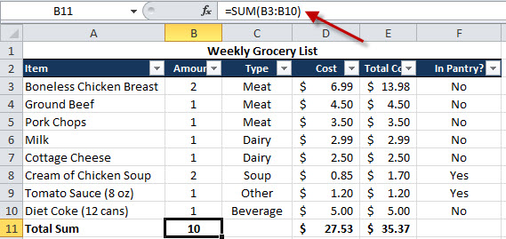
Ok. Now, I would like to show why I love to Filter when using the Subtotal function, but let me first show you the Sum function. Most everyone that uses Excel is familiar with the Sum function. I have added another row to sum up the total # of Items, the Cost and the Total Cost columns. As you can see in the picture below (the arrow is pointing to the actual sum formula I'm using).
This Sum would not change even if I filtered my data. This might be helpful depending on the circumstance, but I like to use the Subtotal function so if I filter my data the Subtotals chang based on what is filtered. In the picture below I have added a new Subtotal row, just like Sum, but using the Subtotal function (the red arrow shows the actual function).

As you can see from my formula it has a number "9" included. When using the subtotal function you have to specify what type of function you want the subtotal to perform. In this case I'm using the Sum function which is number 9.

Ok, so I've added my Subtotal row and I've added the subtotal Sum function to cell B12 and I've added the subtotal Count function to F12 to tell me how many items I will be purchasing. Then, I filtered on "In Pantry?" and selected "No" so I know which Items I need to purchase.

As you can see the "Total Sum" row which uses the normal sum still says 10, whereas the Subtotal Sum has changed to 7. That is because the subtotal only sums those that have been filtered and the Sum function sums all. Now, if you look at Cost and Total Cost you can see the difference based on the Sum and Subtotal function. Then, for column F I used Count and Subtotal Count. So, there are 8 total items in that column, but only 6 have been filtered.
Please let me know if you read my post and if you found it helpful. Also, feel free to requests items you would like me to show you. Have a great night!
2 comments:
OK, WOW that was super, I am in awe and trying to figure how I could use this with quickbooks because I export reports to Excel so I can take out rows and columns - does this sound like something "filtering" would do?
Yes, you can use filtering to remove (or delete) rows. I will do a follow-up post on how to do that. You can't really remove columns though using a filter since the filter deals with rows and not columns.
Post a Comment